For the regression analysis, we are going to use USArrests data that we coveredin class. We will omit the description of the data because it was covered in class.
data("USArrests")
summary(USArrests)
     Murder          Assault         UrbanPop          Rape
 Min.   : 0.800   Min.   : 45.0   Min.   :32.00   Min.   : 7.30
 1st Qu.: 4.075   1st Qu.:109.0   1st Qu.:54.50   1st Qu.:15.07
 Median : 7.250   Median :159.0   Median :66.00   Median :20.10
 Mean   : 7.788   Mean   :170.8   Mean   :65.54   Mean   :21.23
 3rd Qu.:11.250   3rd Qu.:249.0   3rd Qu.:77.75   3rd Qu.:26.18
 Max.   :17.400   Max.   :337.0   Max.   :91.00   Max.   :46.00
How many observations in the dataset?
A) 50
B) 51
C) 52
D) 53
How many variables in the dataset?
A) 3
B) 4
C) 5
D) 6
Crimes like Assault, Murder, and Rape are more likely to happen in cities. Linear regression analysis was performed to find out which variable among Assault, Murder, and Rape was the most Urban-population dependent variable. (See the code below)
Call:
lm(formula = Assault ~ UrbanPop, data = USArrests)

Residuals:
    Min      1Q  Median      3Q     Max
-150.78  -61.85  -18.68   58.05  196.85

Coefficients:
            Estimate Std. Error t value Pr(>|t|)
(Intercept)  73.0766    53.8508   1.357   0.1811
UrbanPop      1.4904     0.8027   1.857   0.0695 .
---
Signif. codes:  0 '***' 0.001 '**' 0.01 '*' 0.05 '.' 0.1 ' ' 1

Residual standard error: 81.33 on 48 degrees of freedom
Multiple R-squared:  0.06701,   Adjusted R-squared:  0.04758
F-statistic: 3.448 on 1 and 48 DF,  p-value: 0.06948
summary(m2)
Call:
lm(formula = Murder ~ UrbanPop, data = USArrests)

Residuals:
   Min     1Q Median     3Q    Max
-6.537 -3.736 -0.779  3.332  9.728

Coefficients:
            Estimate Std. Error t value Pr(>|t|)
(Intercept)  6.41594    2.90669   2.207   0.0321 *
UrbanPop     0.02093    0.04333   0.483   0.6312
---
Signif. codes:  0 '***' 0.001 '**' 0.01 '*' 0.05 '.' 0.1 ' ' 1

Residual standard error: 4.39 on 48 degrees of freedom
Multiple R-squared:  0.00484,   Adjusted R-squared:  -0.01589
F-statistic: 0.2335 on 1 and 48 DF,  p-value: 0.6312
summary(m3)
Call:
lm(formula = Rape ~ UrbanPop, data = USArrests)

Residuals:
    Min      1Q  Median      3Q     Max
-18.644  -5.476  -1.216   5.885  27.937

Coefficients:
            Estimate Std. Error t value Pr(>|t|)
(Intercept)  3.78707    5.71128   0.663    0.510
UrbanPop     0.26617    0.08513   3.127    0.003 **
---
Signif. codes:  0 '***' 0.001 '**' 0.01 '*' 0.05 '.' 0.1 ' ' 1

Residual standard error: 8.626 on 48 degrees of freedom
Multiple R-squared:  0.1692,    Adjusted R-squared:  0.1519
F-statistic: 9.776 on 1 and 48 DF,  p-value: 0.003001
Which dependent variable has the most significant relationship (at least p<0.05) with the urban population?
A) Assault
B) Murder
C) Rape
Choose a model in which only the intercept is a statistically significant coefficient.
A) m1
B) m2
C) m3
According to the result from summary, choose the model that fits the most.
A) m1
B) m2
C) m3
This time, I thought that Murder was influenced by Assault, Rape, and UrbanPop, so I performed the following regression analysis. (Multiple regression, see the code below).
Call:
lm(formula = Murder ~ Assault + Rape + UrbanPop, data = USArrests)

Residuals:
    Min      1Q  Median      3Q     Max
-4.3990 -1.9127 -0.3444  1.2557  7.4279

Coefficients:
             Estimate Std. Error t value Pr(>|t|)
(Intercept)  3.276639   1.737997   1.885   0.0657 .
Assault      0.039777   0.005912   6.729 2.33e-08 ***
Rape         0.061399   0.055740   1.102   0.2764
UrbanPop    -0.054694   0.027880  -1.962   0.0559 .
---
Signif. codes:  0 '***' 0.001 '**' 0.01 '*' 0.05 '.' 0.1 ' ' 1

Residual standard error: 2.574 on 46 degrees of freedom
Multiple R-squared:  0.6721,    Adjusted R-squared:  0.6507
F-statistic: 31.42 on 3 and 46 DF,  p-value: 3.322e-11
Which variable has a statistically significant effect on Y (dependent variable) among X (independent variables)? (at least p<0.05)
A) Assault
B) Rape
C) UrbanPop
Use m4 (above model) to predict the Murder of a new state. New state is Assault=100, Rape=20, UrbanPop=60. Choose the correct predicted Murder of the new state.
A) 3.10
B) 5.20
C) 7.10
D) 9.20
After running the model, you notice that the R-squared is quite high, but the Adjusted R-squared is significantly lower. What could be the most likely reason for this?
A) The model has too many predictors, which might be causing overfitting.
B) The dependent variable is poorly defined.
C) The model has an excellent fit and provides a good predictive power.
D) There is a strong correlation between the predictors and the dependent variable.
Part II. Non-linear Regression
The code below creates a factor-type variable ‘Murder_high’ that is 1 when Murder is greater than 10 (Zero if not), and stores it in USArrests_new.
library(tidyverse)
── Attaching core tidyverse packages ──────────────────────── tidyverse 2.0.0 ──
✔ dplyr     1.1.4     ✔ readr     2.1.5
✔ forcats   1.0.0     ✔ stringr   1.5.1
✔ ggplot2   3.5.1     ✔ tibble    3.2.1
✔ lubridate 1.9.3     ✔ tidyr     1.3.1
✔ purrr     1.0.2
── Conflicts ────────────────────────────────────────── tidyverse_conflicts() ──
✖ dplyr::filter() masks stats::filter()
✖ dplyr::lag()    masks stats::lag()
ℹ Use the conflicted package (<http://conflicted.r-lib.org/>) to force all conflicts to become errors
Choose all states with a predicted probability of being Murder_high is 1 equals 0.5 or greater. (Murder_high가 1일 확률이 0.5보다 큰 것을 고르시오).
A) new_state_1
B) new_state_2
C) new_state_3
Assault’s coefficient in the ‘m5’ model is the log odds ratio. Choose Assault’s Odds ratio.
A) 0.981
B) 1.024
C) 1.038
D) 1.051
Part III. Clustering
Let’s use iris dataset. First thing we need to do for Clustering is the code below.
df <-scale(iris[-5])summary(df)
  Sepal.Length       Sepal.Width       Petal.Length      Petal.Width
 Min.   :-1.86378   Min.   :-2.4258   Min.   :-1.5623   Min.   :-1.4422
 1st Qu.:-0.89767   1st Qu.:-0.5904   1st Qu.:-1.2225   1st Qu.:-1.1799
 Median :-0.05233   Median :-0.1315   Median : 0.3354   Median : 0.1321
 Mean   : 0.00000   Mean   : 0.0000   Mean   : 0.0000   Mean   : 0.0000
 3rd Qu.: 0.67225   3rd Qu.: 0.5567   3rd Qu.: 0.7602   3rd Qu.: 0.7880
 Max.   : 2.48370   Max.   : 3.0805   Max.   : 1.7799   Max.   : 1.7064
Choose the best explanation the reason why we use ‘scale’ before clustering.
A) to minimize the bias caused by different units
B) If you don’t scale, you can’t put it in the clustering function.
C) This is not a necessary procedure
D) to raise the model fit
This is the second step for the k-means clustering.
library(factoextra)
Welcome! Want to learn more? See two factoextra-related books at https://goo.gl/ve3WBa
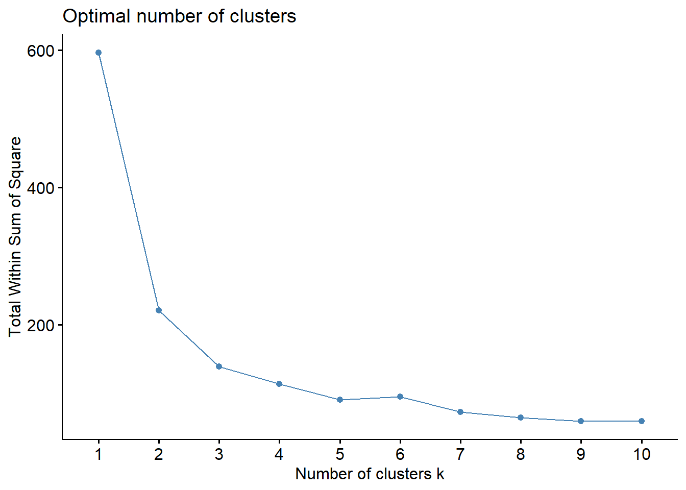
fviz_nbclust(df, kmeans, method ="wss")
See the result, and choose the incorrect explanation of this step.
A) In this step, we can get a recommendation about the number of clusters ‘k’
B) k is bigger the better
C) The appropriate k is 3, but 2 or 4 is also Ok.
D) Total Within Sum of Square is the smallest at k = 10
The code below is k-means clustering with k=3. Then, I created ‘iris_cluster’ by merging the original iris dataset and the clustering result. See the result of the table(iris_cluster\(Species, iris_cluster\)cluster), and answer the questions.
# Compute k-means with k = 3set.seed(123)km.res <-kmeans(df, 3, nstart =25)iris_cluster <-data.frame(iris, cluster = km.res$cluster)table(iris_cluster$Species, iris_cluster$cluster)
As a result of clustering, which species are best divided?
A) Setosa
B) Versicolor
C) Virginica
Let’s get back to the USArrests dataset. You want to group the states into three clusters based on the variables: Assault, Murder, Rape, and UrbanPop. You decide to use K-means clustering to do this.
set of 13 rules

rule length distribution (lhs + rhs):sizes
 2  3
10  3

   Min. 1st Qu.  Median    Mean 3rd Qu.    Max.
  2.000   2.000   2.000   2.231   2.000   3.000

summary of quality measures:
    support         confidence        coverage           lift
 Min.   :0.2308   Min.   :0.4286   Min.   :0.2308   Min.   :0.9286
 1st Qu.:0.2308   1st Qu.:0.5714   1st Qu.:0.3846   1st Qu.:1.2381
 Median :0.2308   Median :0.6667   Median :0.4615   Median :1.4444
 Mean   :0.2663   Mean   :0.6516   Mean   :0.4260   Mean   :1.4020
 3rd Qu.:0.3077   3rd Qu.:0.7500   3rd Qu.:0.4615   3rd Qu.:1.4857
 Max.   :0.3077   Max.   :1.0000   Max.   :0.5385   Max.   :1.9500
     count
 Min.   :3.000
 1st Qu.:3.000
 Median :3.000
 Mean   :3.462
 3rd Qu.:4.000
 Max.   :4.000

mining info:
 data ntransactions support confidence
  txn            13     0.2        0.1
                                                                                       call
 apriori(data = txn, parameter = list(minlen = 2, sup = 0.2, conf = 0.1, target = "rules"))
Choose the incorrect explanations for the result above
A) The highest lift rule is {A,B} => {C}
B) The highest confidence rule is {B,C} => {A}
C) The minimum value of the support is 0.2308
D) Item A and E are highly associated each other
E) lift is the only index we consider to find a good pattern
To increase the sales of item ‘F’, which items should be attached and sold?
A) A
B) B
C) C
D) D
E) E
PART V. Model Comparison and Validation
The following code is the first step we use for the model comparison and validation.
library(caret)
Loading required package: lattice
Attaching package: 'caret'
The following object is masked from 'package:purrr':

    lift
USArrests_new %>%select(-Murder) -> USindexTrain <-createDataPartition(US$Murder_high, p = .9, list = F)training <- US[ indexTrain, ]testing <- US[-indexTrain, ]
Choose the incorrect explanation about the code above.
A) The createDataPartition function is used to divide the dataset into training andtesting dataset.
B) The ratio of training and test data is 7:3.
C) The Murder_high ratio in the train and test sets remains almost the same.
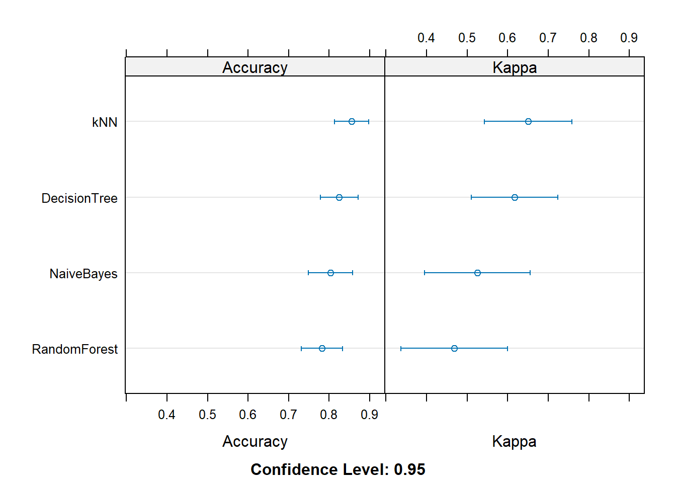
Following code is about training the same dataset with different algorithms (decision tree, random forest, knn, naive bayes), and comparing the model scores.
fitControl <-trainControl(method ="repeatedcv", number =10, repeats =5)dt_fit <-train(Murder_high ~ ., data = training, method ="rpart", trControl = fitControl)rf_fit <-train(Murder_high ~ ., data = training, method ="rf", trControl = fitControl)
note: only 2 unique complexity parameters in default grid. Truncating the grid to 2 .
Choose all incorrect explanations of the code above (multiple choices).
A) To calculate the accuracy and kappa, the repeated cross validation method is used
B) “repeatedcv” divides the training dataset into 5 sections, and validates the model 10times
C) The validation is repeated 5 times overall.
D) Use test dataset for validation.
E) Four models are compared in terms of accuracy and kappa index
Choose the best model according to the graph above
A) kNN
B) Decision Tree
C) Naive Bayes
D) Random Forest
The simplest model, kNN (or decision tree), performed much better than the most complex model, random forest. Which of the following is appropriate for that reason?
A) The number of observations is too small to fit to the complicated model like random forest.
B) This is because the proportion of Y (the dependent variable) = 1 was too small.
C) It’s just a coincidence.
The following code is to predict with dt_fit, using testing dataset. Fill (1) and (2).
Fill (1)
A) testing
B) dt_fit
C) training
D) best_model
Fill (2)
A) training
B) testing
C) repeatedcv
D) dt_fit
You are comparing two models for binary classification (predicting Murder_high), one based on Logistic Regression and the other on a Random Forest. You evaluate their performance using the following metrics:
Model
Accuracy
Kappa
Logistic Regression
0.75
0.50
Random Forest
0.70
0.60
Which model performs better in terms of agreement beyond chance?
A) Logistic Regression, because it has a higher accuracy.
B) Random Forest, because it has a higher Kappa value.
C) Both models perform the same because their accuracies are similar.
D) Random Forest, because it has both higher accuracy and Kappa.
You are evaluating a binary classification model on imbalanced data where 95% of the observations belong to one class. Which metric would be most appropriate to assess the model’s performance?
A) Accuracy
B) Precision
C) Recall
D) F1-Score
Which type of machine learning does not require labeled data?
A) Supervised Learning
B) Reinforcement Learning
C) Unsupervised Learning
D) Semi-Supervised Learning
What is the purpose of cross-validation in machine learning?
A) To split the data into smaller batches for faster training
B) To optimize the hyperparameters of a model
C) To assess the model’s performance by averaging results across multiple subsets of data
D) To create an ensemble of multiple models
Which of the following is NOT an example of supervised learning?
A) Predicting house prices using historical data
B) Identifying fraudulent credit card transactions
C) Grouping customers into segments based on purchasing behavior
D) Diagnosing diseases from medical images using labeled datasets