About me

Computational Social Scientist
Network Scientist
Interdisciplinary Scholar
My research focuses on utilizing computational methods to tackle a wide range of social phenomena, including technology evolution & regional growth, knowledge management, and technology & media innovation. I am passionate about using technology and data to drive innovation and solve real-world problems.
Research
#Innovation#Media#Technology#PublicPolicyTeaching
#DataScience#culture&tech
Introduction

Introduction

Text Mining Techniques
Feature Extraction
Term Frequency-Inverse Document Frequency (TF-IDF)
Weighting words \(W_{(t,d)}\) based on their importance within and across documents to see how the term t is original (or unique) is in a document d
\[ W_{(t,d)}=tf_{(t,d)} \times idf_{(t)} \] \[ W_{(t,d)}=tf_{(t,d)} \times log(\frac{N}{df_{t}}) \]
\(t\) : a term
\(d\) : a document
\(tf_{t,d}\) : frequency of term \(t\) (e.g. a word) in doc \(d\) (e.g. a sentence or an article)
\(df_{term}\) : # of documents containing the term
\(N\) : total number of documents
A high \(tf_{t,d}\) indicates that the term is highly significant within the document, while a high \(df_{t}\) suggests that the term is widely used across various documents (e.g., common verbs). Multiplying by \(idf_{t}\) helps to account for the term’s universality. Ultimately, tf-idf effectively captures a term’s uniqueness and importance, taking into consideration its prevalence across documents.
As an example,
# Calculate the TF-IDF scores
tf_idf <- tokens %>%
count(doc_id, word) %>%
bind_tf_idf(word, doc_id, n)
tf_idf# A tibble: 34 × 6
doc_id word n tf idf tf_idf
<int> <chr> <int> <dbl> <dbl> <dbl>
1 1 academic 1 0.143 1.61 0.230
2 1 important 1 0.143 1.61 0.230
3 1 in 1 0.143 0.511 0.0730
4 1 is 1 0.143 0.916 0.131
5 1 mining 1 0.143 0.916 0.131
6 1 research 1 0.143 1.61 0.230
7 1 text 1 0.143 0.916 0.131
8 2 a 1 0.111 1.61 0.179
9 2 crucial 1 0.111 1.61 0.179
10 2 extraction 1 0.111 1.61 0.179
# ℹ 24 more rows# Spread into a wide format
tf_idf_matrix <- tf_idf %>%
select(doc_id, word, tf_idf) %>%
spread(key = word, value = tf_idf, fill = 0)
tf_idf_matrix# A tibble: 5 × 28
doc_id a academic and animals are cats crucial dogs elephants
<int> <dbl> <dbl> <dbl> <dbl> <dbl> <dbl> <dbl> <dbl> <dbl>
1 1 0 0.230 0 0 0 0 0 0 0
2 2 0.179 0 0 0 0 0 0.179 0 0
3 3 0 0 0.268 0 0.0851 0.268 0 0.268 0
4 4 0 0 0 0.402 0.128 0 0 0 0.402
5 5 0 0 0 0 0.0639 0 0 0 0
# ℹ 18 more variables: extraction <dbl>, feature <dbl>, important <dbl>,
# `in` <dbl>, is <dbl>, large <dbl>, live <dbl>, mammals <dbl>, mining <dbl>,
# ocean <dbl>, pets <dbl>, popular <dbl>, research <dbl>, step <dbl>,
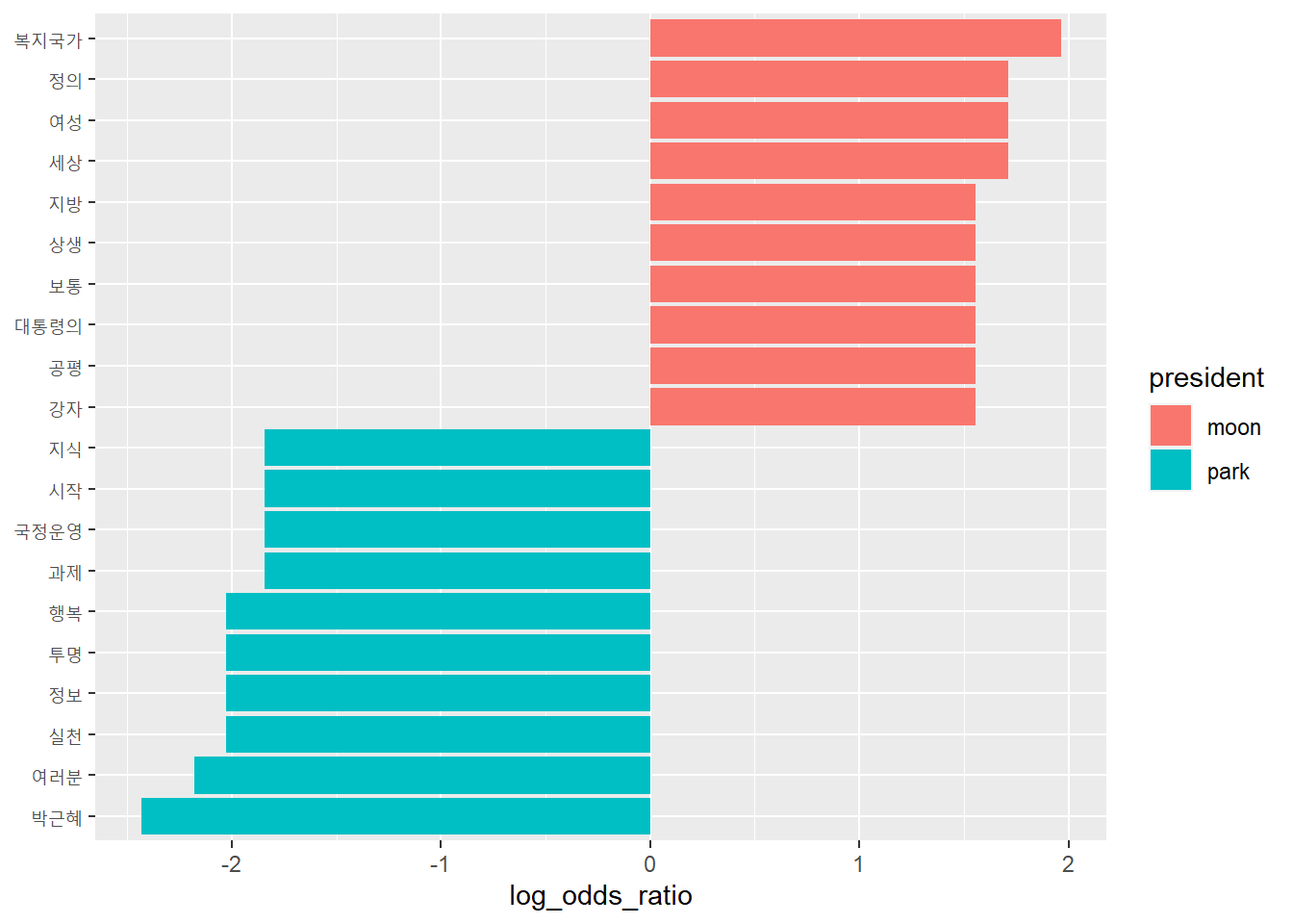
# text <dbl>, that <dbl>, the <dbl>, whales <dbl>Another example: Moon vs. Park speech
- Compare two speeches based on the just frequency of words
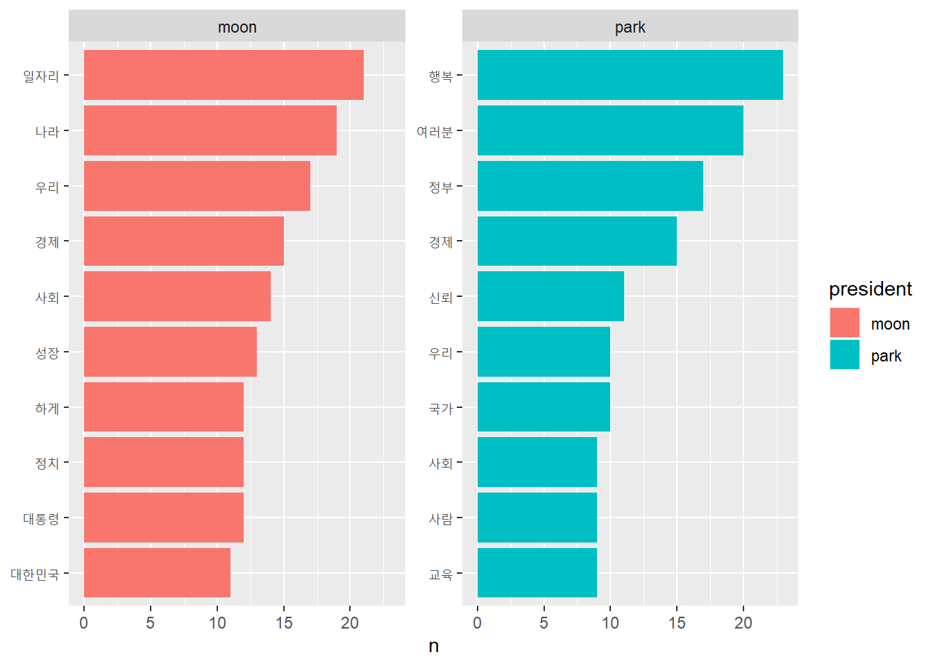
- Compare based on TF-IDF
Text Mining Techniques
Feature Extraction
Word Embeddings
Mapping words to continuous vector spaces based on their semantic relationships

Represents words as fixed-size vectors in continuous space
Captures semantic relationships and linguistic patterns between words
Common algorithms:
Word2Vec,GloVe,FastText→chatGPTPreserves semantic and syntactic properties in high-dimensional vector spaces
Words with similar meanings or usage patterns are closer in vector space
Applications: sentiment analysis, document classification, language translation, information retrieval
Text Mining Techniques
Text Clustering
Partitional clustering method that assigns documents to a fixed number of clusters
Suitable for larger datasets
# A tibble: 5 × 28
doc_id a academic and animals are cats crucial dogs elephants
<int> <dbl> <dbl> <dbl> <dbl> <dbl> <dbl> <dbl> <dbl> <dbl>
1 1 0 0.230 0 0 0 0 0 0 0
2 2 0.179 0 0 0 0 0 0.179 0 0
3 3 0 0 0.268 0 0.0851 0.268 0 0.268 0
4 4 0 0 0 0.402 0.128 0 0 0 0.402
5 5 0 0 0 0 0.0639 0 0 0 0
# ℹ 18 more variables: extraction <dbl>, feature <dbl>, important <dbl>,
# `in` <dbl>, is <dbl>, large <dbl>, live <dbl>, mammals <dbl>, mining <dbl>,
# ocean <dbl>, pets <dbl>, popular <dbl>, research <dbl>, step <dbl>,
# text <dbl>, that <dbl>, the <dbl>, whales <dbl># K-means clustering
set.seed(42)
k <- 3 # Number of clusters
kmeans_model <- kmeans(tf_idf_matrix[, -1], centers = k)
clusters <- kmeans_model$cluster
# Assigning clusters to original data
text_df %>%
mutate(cluster = clusters)# A tibble: 5 × 3
doc_id text cluster
<int> <chr> <int>
1 1 Text mining is important in academic research. 1
2 2 Feature extraction is a crucial step in text mining. 1
3 3 Cats and dogs are popular pets. 2
4 4 Elephants are large animals. 3
5 5 Whales are mammals that live in the ocean. 1Agglomerative clustering method that builds a tree of clusters
Suitable for smaller datasets
# A tibble: 5 × 28
doc_id a academic and animals are cats crucial dogs elephants
<int> <dbl> <dbl> <dbl> <dbl> <dbl> <dbl> <dbl> <dbl> <dbl>
1 1 0 0.230 0 0 0 0 0 0 0
2 2 0.179 0 0 0 0 0 0.179 0 0
3 3 0 0 0.268 0 0.0851 0.268 0 0.268 0
4 4 0 0 0 0.402 0.128 0 0 0 0.402
5 5 0 0 0 0 0.0639 0 0 0 0
# ℹ 18 more variables: extraction <dbl>, feature <dbl>, important <dbl>,
# `in` <dbl>, is <dbl>, large <dbl>, live <dbl>, mammals <dbl>, mining <dbl>,
# ocean <dbl>, pets <dbl>, popular <dbl>, research <dbl>, step <dbl>,
# text <dbl>, that <dbl>, the <dbl>, whales <dbl># Hierarchical clustering
dist_matrix <- dist(tf_idf_matrix[, -1], method = "euclidean")
dist_matrix 1 2 3 4
2 0.5668202
3 0.7631048 0.7491481
4 0.8469394 0.8343861 0.9204641
5 0.6760124 0.6617837 0.7791871 0.8582969
Text Mining Techniques
Text Clustering
Latent Dirichlet Allocation (LDA) (a.k.a. topic modeling)

Text Mining Techniques
Text Clustering
Latent Dirichlet Allocation (LDA) (a.k.a. topic modeling)

Text Mining Techniques
Text Clustering
Latent Dirichlet Allocation (LDA) (a.k.a. topic modeling)

Text Mining Techniques
Text Clustering
Latent Dirichlet Allocation (LDA) (a.k.a. topic modeling)

Text Mining Techniques
Sentiment Analysis
Utilize pre-defined lists of words with associated sentiment scores
Calculate overall sentiment by aggregating scores of individual words
# A tibble: 34 × 2
   doc_id word
    <int> <chr>
 1      1 text
 2      1 mining
 3      1 is
 4      1 important
 5      1 in
 6      1 academic
 7      1 research
 8      2 feature
 9      2 extraction
10      2 is
# ℹ 24 more rows
# Sentiment analysis using NRC lexicon
sentiments_nrc <- tokens %>%
inner_join(get_sentiments("nrc"), by = "word")
sentiments_nrc# A tibble: 7 × 3
doc_id word sentiment
<int> <chr> <chr>
1 1 important positive
2 1 important trust
3 1 academic positive
4 1 academic trust
5 2 feature positive
6 2 crucial positive
7 2 crucial trust sentiments_nrc %>%
group_by(doc_id, sentiment) %>%
count(sentiment) %>%
ggplot(aes(x = as.factor(doc_id),
y = n, fill = sentiment)) +
geom_bar(stat = 'identity',
position = 'fill') +
labs(x = "Document", y = NULL) +
theme_bw()
Train a supervised machine learning model on labeled sentiment data
Apply the trained model to predict sentiment of new text
# A tibble: 5 × 28
  doc_id     a academic   and animals    are  cats crucial  dogs elephants
   <int> <dbl>    <dbl> <dbl>   <dbl>  <dbl> <dbl>   <dbl> <dbl>     <dbl>
1      1 0        0.230 0       0     0      0       0     0         0
2      2 0.179    0     0       0     0      0       0.179 0         0
3      3 0        0     0.268   0     0.0851 0.268   0     0.268     0
4      4 0        0     0       0.402 0.128  0       0     0         0.402
5      5 0        0     0       0     0.0639 0       0     0         0
# ℹ 18 more variables: extraction <dbl>, feature <dbl>, important <dbl>,
#   `in` <dbl>, is <dbl>, large <dbl>, live <dbl>, mammals <dbl>, mining <dbl>,
#   ocean <dbl>, pets <dbl>, popular <dbl>, research <dbl>, step <dbl>,
# text <dbl>, that <dbl>, the <dbl>, whales <dbl># Train a Random Forest model
train_data <- tf_idf_matrix %>%
left_join(sentiments_nrc, by = "doc_id") %>%
relocate(sentiment, .after = doc_id) %>%
drop_na %>%
select(-doc_id)
train_data# A tibble: 7 × 29
sentiment a academic and animals are cats crucial dogs elephants
<chr> <dbl> <dbl> <dbl> <dbl> <dbl> <dbl> <dbl> <dbl> <dbl>
1 positive 0 0.230 0 0 0 0 0 0 0
2 trust 0 0.230 0 0 0 0 0 0 0
3 positive 0 0.230 0 0 0 0 0 0 0
4 trust 0 0.230 0 0 0 0 0 0 0
5 positive 0.179 0 0 0 0 0 0.179 0 0
6 positive 0.179 0 0 0 0 0 0.179 0 0
7 trust 0.179 0 0 0 0 0 0.179 0 0
# ℹ 19 more variables: extraction <dbl>, feature <dbl>, important <dbl>,
# `in` <dbl>, is <dbl>, large <dbl>, live <dbl>, mammals <dbl>, mining <dbl>,
# ocean <dbl>, pets <dbl>, popular <dbl>, research <dbl>, step <dbl>,
# text <dbl>, that <dbl>, the <dbl>, whales <dbl>, word <chr>model_rf <- rpart("sentiment ~ a + academic + crucial",
data = train_data)
# Predict sentiment for new text
predictions <- predict(model_rf, newdata = tf_idf_matrix)
predictions positive trust
[1,] 0.5714286 0.4285714
[2,] 0.5714286 0.4285714
[3,] 0.5714286 0.4285714
[4,] 0.5714286 0.4285714
[5,] 0.5714286 0.4285714Train a deep learning model, such as a Recurrent Neural Network (RNN) or Transformer, on labeled sentiment data
Apply the trained model to predict sentiment of new text
Text Mining Techniques
Relation Extraction
- A. Preprocessing and extracting keywords
- B. Co-occurrence matrix and network
- C. Analyzing keyword network
Tokenization
Stop word removal
Stemming or lemmatization (optional)
Sample text: 6 sentences
Text mining and data mining are essential techniques in data science, and they help analyze large amounts of textual data. Machine learning, natural language processing, and deep learning are crucial techniques for text mining and data analysis. Text mining can reveal insights in large collections of documents, uncovering hidden patterns and trends. Big data analytics involves data mining, machine learning, text mining, and statistical analysis. Sentiment analysis is a popular application of text mining, natural language processing, and machine learning, often used for social media analytics. Data visualization plays a significant role in understanding patterns and trends in data mining results, making complex information more accessible.
# Example dataset
text_data <- tibble(
  doc_id = 1:6,
  text = c("Text mining and data mining are essential techniques in data science, and they help analyze large amounts of textual data.",
           "Machine learning, natural language processing, and deep learning are crucial techniques for text mining and data analysis.",
           "Text mining can reveal insights in large collections of documents, uncovering hidden patterns and trends.",
           "Big data analytics involves data mining, machine learning, text mining, and statistical analysis.",
           "Sentiment analysis is a popular application of text mining, natural language processing, and machine learning, often used for social media analytics.",
           "Data visualization plays a significant role in understanding patterns and trends in data mining results, making complex information more accessible.")
)
text_data
# A tibble: 6 × 2
doc_id text
<int> <chr>
1 1 Text mining and data mining are essential techniques in data science, …
2 2 Machine learning, natural language processing, and deep learning are c…
3 3 Text mining can reveal insights in large collections of documents, unc…
4 4 Big data analytics involves data mining, machine learning, text mining…
5 5 Sentiment analysis is a popular application of text mining, natural la…
6 6 Data visualization plays a significant role in understanding patterns …# Tokenization
tokens <- text_data %>%
unnest_tokens(word, text) %>%
anti_join(stop_words) %>%
group_by(doc_id) %>%
count(word, sort = TRUE)
tokens# A tibble: 67 × 3
# Groups: doc_id [6]
doc_id word n
<int> <chr> <int>
1 1 data 3
2 1 mining 2
3 2 learning 2
4 4 data 2
5 4 mining 2
6 6 data 2
7 1 amounts 1
8 1 analyze 1
9 1 essential 1
10 1 science 1
# ℹ 57 more rowsCalculate word co-occurrence matrix
Convert co-occurrence matrix to a graph object
Visualize the keyword network
# Calculate co-occurrence matrix
co_occurrence_matrix <- tokens %>%
  ungroup() %>%
  pairwise_count(word, doc_id, sort = TRUE)

co_occurrence_matrix
# A tibble: 586 × 3
item1 item2 n
<chr> <chr> <dbl>
1 text mining 5
2 mining text 5
3 mining data 4
4 data mining 4
5 text data 3
6 learning mining 3
7 analysis mining 3
8 machine mining 3
9 mining learning 3
10 text learning 3
# ℹ 576 more rows# Filter edges and create graph object
filtered_edges <- co_occurrence_matrix %>%
filter(n >= 2)
keyword_network <- graph_from_data_frame(filtered_edges)
keyword_networkIGRAPH 0350ef0 DN-- 13 88 --
+ attr: name (v/c), n (e/n)
+ edges from 0350ef0 (vertex names):
[1] text ->mining mining ->text mining ->data
[4] data ->mining text ->data learning ->mining
[7] analysis ->mining machine ->mining mining ->learning
[10] text ->learning analysis ->learning machine ->learning
[13] data ->text learning ->text analysis ->text
[16] machine ->text mining ->analysis learning ->analysis
[19] text ->analysis machine ->analysis mining ->machine
[22] learning ->machine text ->machine analysis ->machine
+ ... omitted several edges# Visualize the keyword network
ggraph(keyword_network, layout = "fr") +
geom_edge_link(aes(edge_alpha = n), show.legend = FALSE) +
geom_node_point(color = "blue", size = 5) +
geom_node_text(aes(label = name), vjust = 1, hjust = 1, size = 10) +
theme_graph(base_family = "Arial") +
labs(title = "Keyword Co-occurrence Network")
To understand the graph better, let’s examine some of the connections:
text -> mining: The keyword ‘text’ is connected to the keyword ‘mining’. This edge represents that ‘text’ and ‘mining’ co-occur in the dataset, forming the term ‘text mining’.mining -> data: The keyword ‘mining’ is connected to the keyword ‘data’, indicating that these two terms appear together, forming the term ‘data mining’.learning -> machine: The keyword ‘learning’ is connected to the keyword ‘machine’, representing the co-occurrence of these two terms, forming ‘machine learning’.analysis -> text: The keyword ‘analysis’ is connected to the keyword ‘text’, suggesting that these two terms co-occur in the dataset, forming the term ‘text analysis’.
From this graph, you can observe the following:
Keywords related to data analysis techniques, such as ‘text mining’, ‘data mining’, ‘machine learning’, and ‘analysis’, are strongly connected, indicating that they are frequently discussed together in the dataset.
The term ‘text mining’ is connected to ‘data mining’, ‘machine learning’, and ‘analysis’, suggesting that these techniques are closely related and are often mentioned in the context of text analysis.
The term ‘machine learning’ is connected to ‘text mining’, ‘data mining’, and ‘analysis’, highlighting its importance and relevance to different data analysis techniques.
Degree centrality: Number of connections for each nodeBetweenness centrality: Importance of a node as a connector in the networkCommunity detection: Clustering of nodes in the network
# Degree centrality
degree_centrality <- degree(keyword_network)
# Betweenness centrality
betweenness_centrality <- betweenness(keyword_network)

tibble(node = names(degree_centrality),
       degree_centrality = degree(keyword_network)) %>%
  left_join(
    tibble(node = names(degree_centrality),
       betweenness_centrality = betweenness(keyword_network))
  ) -> node_data
node_data
# A tibble: 13 × 3
node degree_centrality betweenness_centrality
<chr> <dbl> <dbl>
1 text 20 8.8
2 mining 24 48.8
3 data 12 2
4 learning 18 2.8
5 analysis 18 2.8
6 machine 18 2.8
7 techniques 6 0
8 language 14 0
9 natural 14 0
10 processing 14 0
11 patterns 4 0
12 trends 4 0
13 analytics 10 0 # Degree - Btw mat
node_data %>%
ggplot(aes(x = degree_centrality,
y = betweenness_centrality)) +
geom_text_repel(aes(label = node), size = 10)
# Degree - Btw mat (2)
node_data %>%
  filter(betweenness_centrality < 7) %>%
  ggplot(aes(x = degree_centrality,
             y = betweenness_centrality)) +
  geom_text_repel(aes(label = node), size = 10)
# Community detection using Louvain method

# Convert the directed graph to an undirected graph
undirected_keyword_network <- as.undirected(keyword_network, mode = "collapse")

# Perform community detection using the Louvain algorithm
louvain_communities <- cluster_louvain(undirected_keyword_network)

# Print the community assignments
print(louvain_communities)
IGRAPH clustering multi level, groups: 3, mod: 0.1
+ groups:
$`1`
[1] "text" "data" "techniques"
$`2`
[1] "mining" "patterns" "trends"
$`3`
[1] "learning" "analysis" "machine" "language" "natural"
[6] "processing" "analytics"
# Visualize the keyword network with community colors
ggraph(keyword_network) +
  geom_edge_link(aes(width = n), alpha = 0.5) +
  geom_node_point(aes(size = degree_centrality,
                      col = louvain_communities_char)) +
  geom_node_text(aes(label = name, color = louvain_communities_char),
                 vjust = 1.5, hjust = 1.5,
                 size = 10) +
  scale_color_discrete(name = "Community") +  # add a legend for community colors
  theme_graph(base_family = "Arial") +
  labs(title = "Keyword Network with Community Detection")
Applications in Academic Research

Applications in Academic Research

Applications in Academic Research

Conclusion and Future Directions
D. Addressing challenges and limitations for more robust applications:
Tackling unstructured and noisy data: Developing techniques to better handle, clean, and preprocess unstructured and noisy data will improve the accuracy and reliability of text mining applications in academic research.
Addressing ethical and legal concerns: Researchers must continue to engage in discussions and develop guidelines to address data privacy, copyright, and intellectual property issues related to text mining.
Improving scalability and computational efficiency: As the volume of data continues to grow, researchers need to develop more scalable and computationally efficient text mining techniques to handle large-scale datasets and real-time processing demands.